Background:

From the end of May conditions across Europe begin to become favourable for the development of severe thunderstorms. This can occur in many different ways, though one of the more well-known and common modes is the 'Spanish Plume', which despite its name, is a meteorological process that can originate from airmasses over North Africa, as well as the more recognised plumes that affect the UK and originate from the Meseta Central in Spain, where it derives its name from.

Very warm or hot and dry air that forms in North Africa, or over the Iberian plateau, is drawn north in the backing (anticlockwise) upper flow that develops in advance of an extending upper trough out in the Northeast Atlantic. This increasingly meridional flow transports this hot and dry air further and further north, ascending as it does so through isentropic upgliding/strong thermal advection, with it already having some altitude having originated over relatively modest high ground. This creates an elevated mixed layer (EML), typically characterised by high potential temperature with steep lapse-rates approaching a DALR (Dry Adiabatic Lapse Rate of 9.8K / km), which along with the cooling that occurs at lower levels in the higher latitudes that it drifts towards, has the effect of capping the boundary layer.

This environment is sometimes described as the classic 'loaded gun' type profile, where heat is able to build beneath the strong capping inversion without releasing any of the CAPE (Convective Available Potential Energy) that lies above. If sufficient heat and moisture is added to the boundary layer, or some external forcing helps to erode the cap, then all of the CAPE can be released at once and produce a large and potentially severe thunderstorm, owing to the steep lapse rates in the EML.

Storm Mode and Severity:

The severity and type of storm mode is dictated by a delicate balance between the amount of CAPE and vertical wind shear in the lowest few km of the atmosphere. Where these two balance precisely the most severe thunderstorm mode, the 'supercell' can develop. If there is too much shear in an environment where only small amounts of CAPE exist, potential storms are simply torn apart well before developing significant organisation; or in some cases where there is modest CAPE and large shear they can develop into NCFRs (Narrow Cold Frontal Rain bands), which can be the most common cause of tornadoes in the UK.

High CAPE in low vertical wind shear environments tends to produce short-lived pulse storms/cells that cannot become organised and rain themselves out. This is because the downdraught does not become tilted, which leads to it effectively killing or cutting off the inflow of the developing storm. A subtle balance is required with increasing CAPE supported by increasing amounts of vertical wind shear to help provide the perfect ingredients, this is typically found to be a Bulk Richardson Number (ratio related to the consumption of turbulence divided by the shear production of turbulence) of between 15 and 40, anything significantly above 40 generally indicates less severe convection is likely. This number is available on Visual Weather tephigrams for quick assessment.

Case Study - NE France, Belgium/Netherlands/Luxembourg, 4 June 2019

The WV (Water Vapour) and 300hPa Geopotential Height loop hows the extending upper trough across to the west of the UK, with the jet clearly defined running SSW to NNE across NE France and through SW England, with its exit located across southern Scotland. To the east of the jet, upstream of the ridge axis there was a plume extending northward, indicated at 700hPa by a narrow plume of >16C Wet Bulb Potential Temperature (see Figure 2, right). On the edge of this plume storms were initiated soon after 15 Z in the boundary layer across NE France, and then continued to develop widely across the Netherlands, Belgium and Luxembourg before upscaling into a large MCS that continued north across southern North Sea and towards Denmark and Norway, broadly following the mid-level steering flow.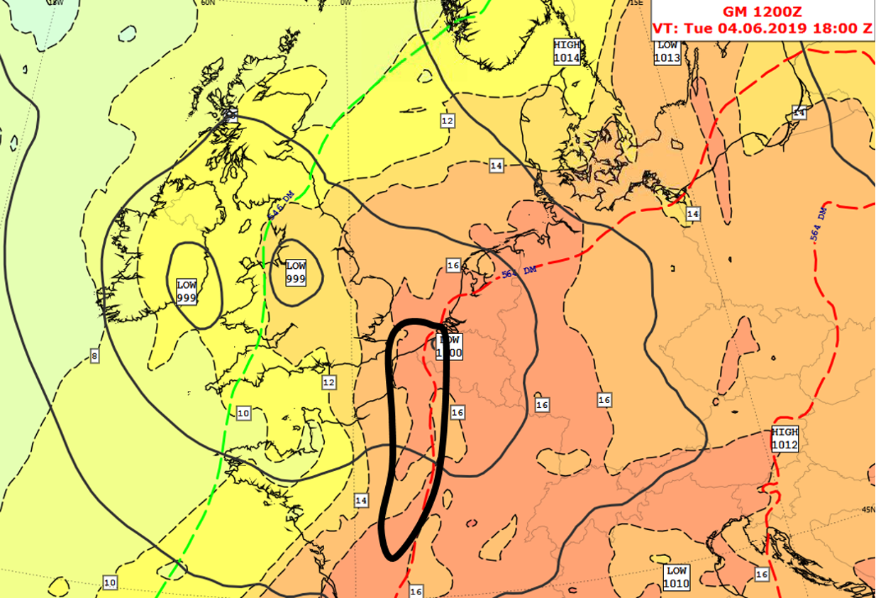

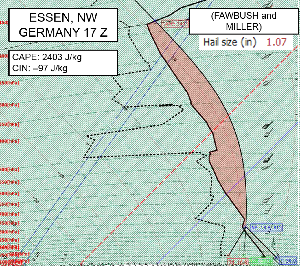
An actual radiosonde ascent from Essen in NW Germany at 17 Z (see Figure 3, left), slightly forward of the main plume shows how unstable the atmosphere is. Modifying the ascent slightly to give the observed conditions from the area near where convection initially broke out, suggests that a very large amount of CAPE is likely to be released.

The EML is clearly discernible above around 800 hPa, and the small capping inversion appears to have become eroded, this allowing the release of large amounts of CAPE once that capping inversion could be overcome, aided further by the development of convection which cool this layer. Further to this, there is a modest amount of shear in the lowest few km, this is limited to the lowest 1.5km, below around 850 hPa.

The Bulk Richardson number from this ascent was near to 10, which is close to the number required for the development of severe organised convection, but suggests that shear of around 45–50 knots slightly dominated over CAPE and this may have organised the convection into a weak derecho (which is a form of squall or straight-line wind storm, capable of damaging gusts).

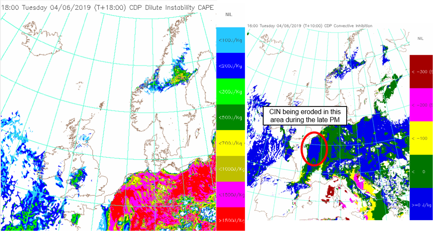
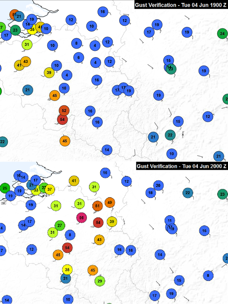
The CAPE value calculated from the construction in Figure 3 (2403 J/kg) is an overestimate that fails to account for, among other things, processes such as entrainment. More realistic values of the order 1000–1500 J/kg forecast by the Euro 4 model over the area of interest (see Figure 4, below). These figures of 1500 J/kg are very high for the more temperate regions of NW Europe and are another clear sign of the potential for severe convection. Associated with the thunderstorms there were some significant gusts recorded of the order 50 to 55 knots, locally 60 knots (see Figure 5, below left, which shows reported gusts at 19 Z and 20 Z across the area where convection broke out). In this next part of this blog we will consider two different empirical techniques that have been shown to provide a reasonable “rough” first estimate in such situations, though it is worth noting that these techniques fail to consider processes such as precipitation loading and will struggle to provide anything but a rough approximation to the processes involved, especially when forecasting MCSs.

Ivens and Fawbush & Miller Empirical Techniques

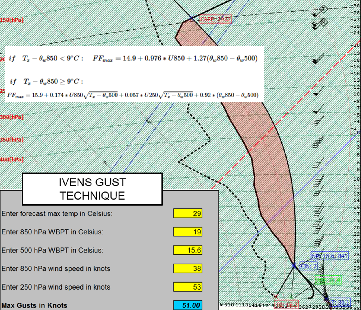
This blog will now look at a number of different empirical techniques that can be utilised by meteorologists. The first is the Ivens method (developed 1987), this has been used by the forecasters at KNMI in the Netherlands to predict the maximum wind velocity associated with heavy showers or thunderstorms. The method of Ivens is based on two multiple regression equations that were derived using about 120 summertime cases (April to September). The amount of negative buoyancy, which is estimated in these equations by the difference of the potential wet-bulb temperature at 850 and at 500 hPa, and horizontal wind velocities at one or two fixed altitudes, used to determine the potential amount of momentum aloft available, are used to estimate the maximum wind velocity.

Although the method of Ivens has been designed for summertime situations, forecasters at KNMI apply the method throughout the year on profiles from NWP models. In this case (see Figure 6, below) the Ivens technique provides an estimate of maximum gust of the order 51 knots. This is quite close to the observed maximum gusts and a reasonable estimate of the likely maximum convective gust associated with most active cells.

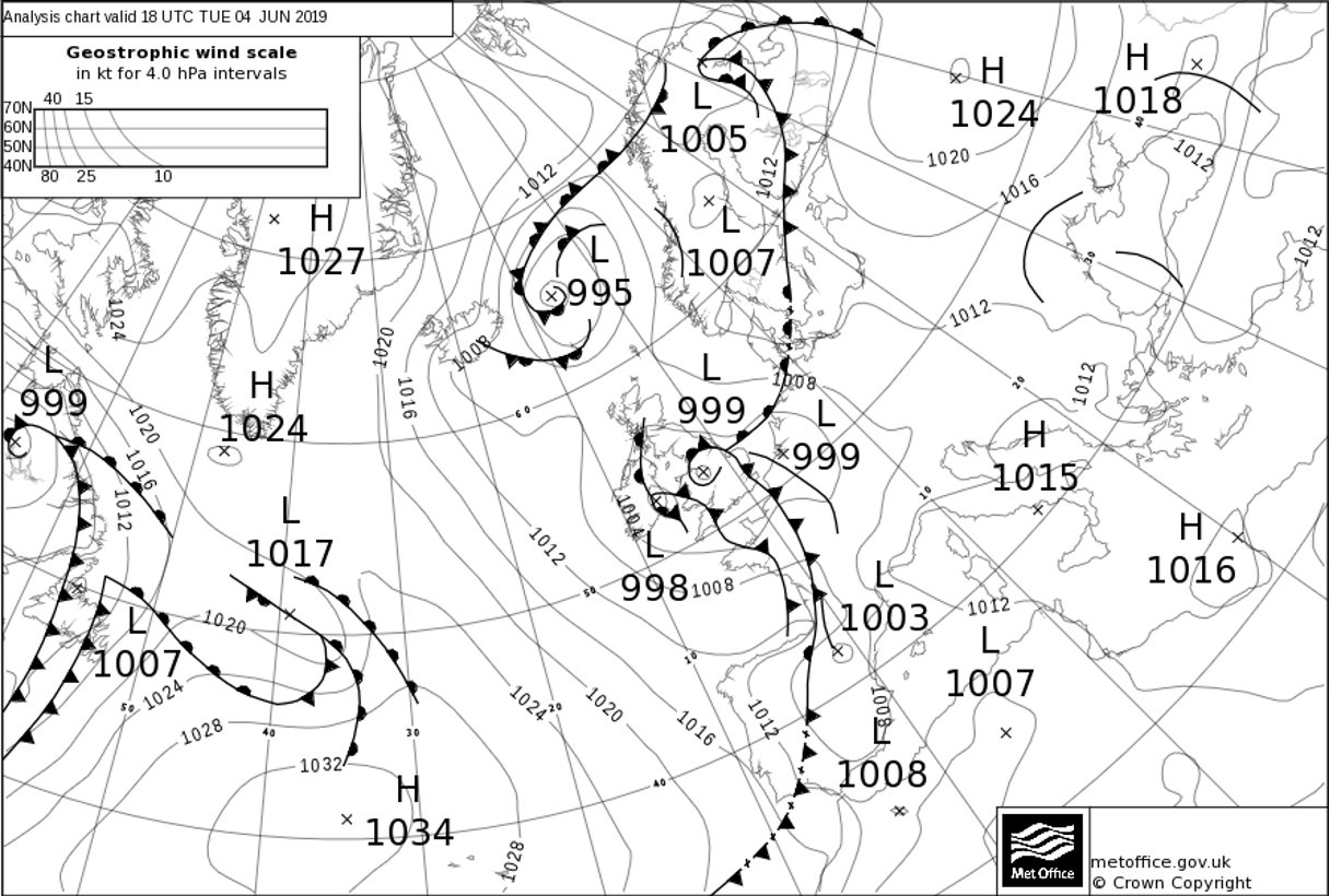
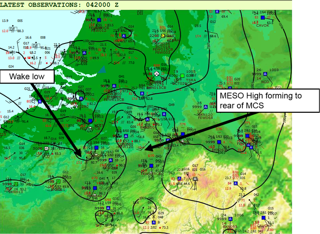
It was notable from the surface pressure analysis (see Figure 7, below right) that a “meso high” had formed immediately ahead of the line of developing and active cells, with a “wake low” following yet further behind. This “meso high” disrupts the surface isobaric pattern markedly, and is typically associated with severe convection and MCS development. It develops in the rain cooled outflow region of the storm, and its magnitude is dependent on the strength of the cold pool outflow associated with the storm. Isallobaric analysis shows a marked couplet and tight gradient in the vicinity of the convective activity and perpendicular to the convective gust direction, suggesting a marked ageostrophic component to the wind.

Fawbush and Miller methods for gusts and hail size

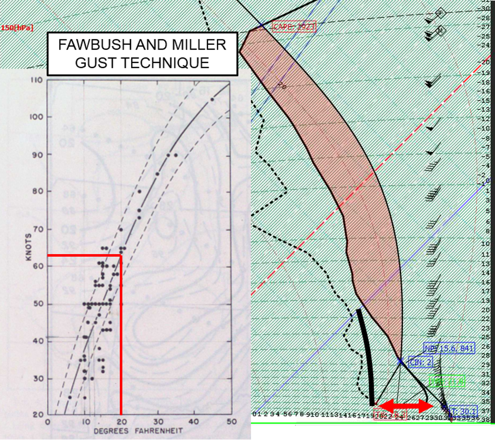
Another technique that is considered here is the Fawbush and Miller method (1954), two meteorologists who issued the first ever tornado warning in 1948. This technique relates the maximum gust strength to the potential negative buoyancy force in a convective downdraught, essentially the strength depends largely on the temperature difference between the rain cooled downdraught in the thunderstorm outflow, and the surrounding warmer ambient airmass in which the storms develop. Whilst this method was empirically derived in the United States where it is more applicable, it has been found to be useful for summertime severe convection, especially across Europe – whereas in the UK its use is limited, primarily because downward transfer of momentum typically dominates, and this is not considered by this technique. However, it has been found to have some usefulness in the most extreme UK case studies.

This technique (see Figure 8, below) uses an SALR (Saturated Adiabatic Lapse Rate) from the Wet Bulb Zero level to the surface as a proxy for the “downdraught temperature” and then compares this to the ambient temperature outside the thunderstorms to determine the strength of peak gusts. Note this is for a maximum gust, and that typically measured gusts will be below this value, therefore it is to be used as a forecast “worst case scenario”. In this example, this suggested a “downdraught temperature” of approximately 18 degrees Celsius and the temperature outside of thunderstorms peaked at between 29 and 30 degrees Celsius – a differential of 11 degrees (or 20 degrees Fahrenheit) which gives a peak gust of 62–63 knots (with a range of between 55 and 70 knots).

Again, noting the caveats above, this technique also provides a reasonable estimate of the potential maximum gusts realised in this severe convection. The highest recorded gust was 68 knots at Huibertgat.

Finally, there is also a Fawbush and Miller technique for calculating hail size (1953) which is used in the post-processed GPP output and also is included within the tephigram convective parameters on Visual Weather (under “Thermodynamic Indices”). This technique considers updraught strength (from CAPE between the cloud base and the MS05 degree isotherm) and the depth of cloud below the MS05 degrees isotherm. Provided that the cloud top is colder than MS18 to MS20 then this technique can give an approximation of maximum hail size. Note that the technique fails to consider shear, which is arguably a larger and certainly a significant contributor to the development of large hail.

In this example (see Figure 3) the hail size predicted by this Fawbush and Miller technique suggested a maximum hail size of around 1 inch. Hail reports from across the Netherlands (see Figure 9) suggested hail of around 2-2.5 cm in diameter, which matches very well with the forecast from this technique.

Summary:

In summary, when considering the development of severe convection and the likelihood of significant impacts such as damaging wind gusts and/or large hail, these "rough and ready" techniques can quite quickly provide the forecaster with a quick approximation of the magnitude of such variables. This enables them to make critical decisions quickly and also whether to spend a greater amount of time looking in more detail at these for a more precise forecast. Though they have limitations and will struggle to represent the complex processes that take place within the most organised deep convection, this particular case study demonstrates that they can still offer reasonable advice.

I am interested in any other techniques that others have come across or found useful, so please feel free to append these techniques and any appropriate links in the comments.

References

Ivens, R. A. A. M.: 1987, Forecasting the maximum wind velocity in squalls. Symp. Mesoscale Analysis and Forecasting, ESA, 685–686.

Ernest J. Fawbush and Robert C. Miller, 1953: A Method for Forecasting Hailstone Size at the Earth's Surface. Bulletin of the American Meteorological Society, 34, 235–244.

Ernest J. Fawbush and Robert C. Miller, 1954: A Basis for Forecasting Peak Wind Gusts in Non-Frontal Thunderstorms. Bulletin of the American Meteorological Society 35, 14–19.